When attempting to comprehend the expansive concept of infinities, it can often be arduous for the human mind to grasp the underlying properties of boundless number sets. The word “infinity” is often superficially used in conversation to imply an unfathomable amount of something. Or, possibly even more widespread, it was popularized by Buzz Lightyear’s famous tagline “To infinity and beyond!”. But was our toy box companion correct? Can we actually go past infinity?
To answer this question, we have to begin by adequately defining the concept of infinity. Surprisingly, it’s not that straightforward. As discussed, hyperbolic rhetoric used casually in conversation can have misleading effects on a person’s perception of infinity — namely, mathematical infinities. Specifically, the idea behind countable and uncountable infinities can appear perplexing at first glance. However, as devised by Georg Cantor in 1891, Cantor’s Diagonal Argument explains the monumental discovery that not all infinities are of the same size. The Argument directly proves that the set of all real numbers is uncountably infinite and thus larger than the set of natural numbers.
Let’s begin by considering a set of all the real numbers between 0 and 1, (0, 1), and suppose that f : N → (0, 1) is an arbitrary function, where N is the set of all natural numbers. Construct a table of values, matching value in N (1, 2, 3, 4, …) to its output, f (n). The values in the f (n) column of the table represent arbitrary decimals between 0 and 1 (there isn’t a “smallest” so we can just have them in any order). For instance, f (1) = 5/17, f (2) = e/100, f (3) = 16/23 are values that could correspond to the first three rows of the table. Evidently, the entire list cannot actually be written down, but a partial representation of the entire table will suffice. However, with the assumption that every number in N has been matched to a number in (0, 1), is the table a conclusive list of all the real numbers between 0 and 1? Shockingly, there are still infinitely many more values in (0, 1) that are not recognized on the table. For instance, consider the predicament of wanting to create a new decimal not shown on the list. To ensure that the new decimal being created never appears on the table, the value can be constructed by slightly changing values on the current table. Specifically, construct the new number by first circling each number that exists on the main diagonal — namely, the diagonal that extends from the first digit (right of the decimal point) of the first row to the second digit of the second row, and continues downward indefinitely. Now, take each circled number and add 1 to it. If a number on the diagonal happens to be a 9, simply subtract 1 instead of adding. The resulting values, when assembled into a decimal represent a unique number, different from any other on the initial list. The newly added decimal is guaranteed to be different from every other table value by at least one number: the number on the diagonal. For example, if the first few rows of the table appeared as shown in the animation below, the resulting decimal would be 0.571909… and after adding/subtracting 1 to each respective digit, the new decimal would begin with 0.682818… which differs from all other values on the table. Impressively, this process can be repeated infinitely by changing the amount added or subtracted from each digit on the diagonal — instead of adding or subtracting 1, the values could be changed by other factors such as adding 5 or subtracting 3 — thus proving that there are an infinite amount of real numbers in the range (0, 1). By contrast, although there may be a corresponding value, f (n), for every value of n, there is not necessarily a value n for every value between 0 and 1. Therefore, there will always be infinitely many missing values that are unrecognized on the table, proving that a bijection does not exist between N and (0, 1).

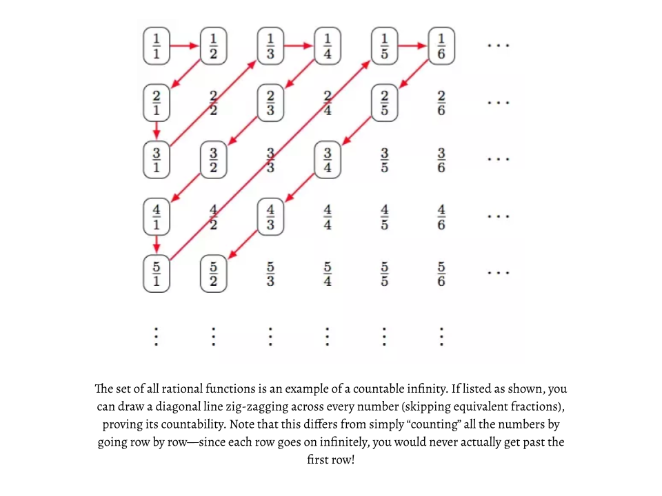
Cantor’s revolutionary Diagonal Argument revealed the disparity in size between infinites, and highlighted the concepts of countable and uncountable infinities. In this proof, the set of natural numbers, N, represents a countable infinity, implying that, although extending to infinity, it is possible to “count” each element in the set. This can simply be done by listing every natural number in existence — despite its impracticality, they are technically countable. Nowadays, this infinity is denoted by the symbol aleph-null:

and is regarded as the first, smallest infinity. However, the set of all real numbers, R, is uncountably infinite, as proven by Cantor’s Argument. There will always be a method to devise a real number that is not listed on the table, thus cementing its uncountability. As it turns out, there are an infinite number of uncountable infinities! Although contentious during its time of release, Cantor’s Diagonal Argument revolutionized mathematics, and offered a new perception of infinity.
Now armed with this powerful knowledge of infinities, we return to the preliminary question: How can we prove Buzz Lightyear to be correct or incorrect in his proclaimed statement? Let’s build off of what we already know—the existence of differently sized infinities. To start, we must define what it means for two sets of numbers to be “equal”. For the purposes of infinity, equality implies that every number in one set can be matched up with a number in another set. Mathematically, this means that a function must be bijective, with a one-to-one correspondence for each input and output. If this condition is met, two sets are considered equivalent. Having a broader definition for “equal”, such as this, gives us the ability to unveil some mind-bending properties of infinities. Let’s look back to Cantor, and see what we can find. The Diagonal Argument is an example of an injective function, meaning that every input (natural number) has exactly one output (real number in the interval (0,1)). However, injectivity does not guarantee that each output corresponds to an input, as highlighted in the Argument. In our proof, we successfully devised an output without a corresponding input, showing that the two sets are neither bijective nor equal. Furthermore, we can also use this definition of equality to state that the set of all even numbers is equal to the set of all natural numbers. Superficially, this seems incorrect—there should be twice as many natural numbers as even numbers, right? However, using the broadly defined version of “equality”, we realize that we can match up every even number to a natural number—there are an infinite amount of both! By a similar logic, the set of odd numbers is also equal to aleph-null (the infinity of the set of all natural numbers). Even more perplexing, 1 + aleph-null = aleph-null, because we can still match up every value in both infinite sets to each other. Since there are infinite amounts of both, adding one has no effect on the value of aleph-null. Thus, the theory that we can count past infinity by simply adding 1 is disproved. Things aren’t looking good for Buzz Lightyear at this point.

But wait! If we proved that there exist infinities of different sizes, then there must be a number that allows us to count past at least one of these infinities. After all, for there to be differently sized infinites, there have to be numbers beyond a smaller infinity that allow us to reach a larger one. We begin once again by understanding how to approach our problem. To achieve a number past infinity, we must first discuss two things, ordinal numbers, and axioms. First off, we can technically count past infinity, that is to say aleph-null, with the use of ordinal numbers. On a daily basis, the numbers we use are known as “cardinal numbers”, as they describe the cardinality, or amount, that a number represents. For instance, 314 pies indicates the quantity of pies that I have. By contrast, ordinal numbers don’t describe the size of numbers, but rather, the order in which they appear. For finite values, cardinality and ordinality are equal; however, after arriving at aleph-null, we need a new symbol to describe the ordinality of what comes after that. This symbol is denoted by ω, and is the first transfinite ordinal. After that comes ω+1, ω+2, ω+3…etc. Note that ω+1 isn’t necessarily a larger value than ω, it just comes after ω—basically, ordinal values describe the order type of a number. The order type of a number is simply the next ordinal number not needed to arrange a set in correct order (an important contingency for order types is that a set must be well-ordered, or in other words, in the correct order). For instance, the order type of the set {1, 2, 3, 4, 5} is 6, and the order type of the natural numbers is ω. By contrast, the set {6, 4, 3, 5, 2, 1} doesn’t have an order type, since it isn’t well-ordered. The importance of order type will be more clear later on in our expedition. Just remember that ω isn’t considered a cardinal number, and cannot be treated as such. Although we have found a representation of a value beyond infinity, we have not yet arrived at a cardinal quantity beyond aleph-null. Our search continues…

Another useful concept that can aid in our journey to “Infinity and Beyond” are axioms—essentially, statements that are said to be true, without the need of a proof to verify their validity. For instance, the existence of aleph-null is an axiom, devised by German mathematician Ernst Zermelo. Let’s go back to our ordinal numbers, which come after the countably infinite quantity of all the natural numbers. If we continue to add 1 to our previous value, we go from ω to ω+1 to ω+2, and onwards, eventually arriving at the monstrous total ω+ω, or 2ω. At this point, we’ve reached yet another ceiling; it is impossible to go past this point without the use of more axioms. An invaluable axiom that can be of use is the Axiom Schema of Replacement, which allows us to replace previously reached values with new ones, while still maintaining our set. Basically, armed with this axiom, we can now replace every ordinal value up to ω with ω x (ordinal value), which eventually leads us to the value of ωω. Continuing this process, by repeatedly replacing previously achieved values with larger ones, we arrive at ω to the ωth power to the ωth power to the ωth power to the ωth power to the ωth power to the… where we run out of standard notation to use to express this quantity. To sidestep such an issue, this value is simply referred to as ε0 (“epsilon-not”). Ridiculously enough, we can keep going. Past ε0, we can continue to list more and more ordinal values—all the different ways to list an aleph-null amount of things. And then we realize… that the list of all of these different ordinal numbers will have an order type. That is to say, that there exists an ordinal number beyond the set of ordinal numbers discussed. After all, the set of all of these ordinal numbers is well-ordered. This new ordinal number is written as ω1, and it has a corresponding cardinal number denoted as aleph-one. This is a huge deal! Although aleph-one may not represent any “normal” number like 25, 203321, or 2.72, it still proves the existence of a value larger than infinity, albeit the requirement of the belief in an even larger infinity. The understanding of aleph-one opens the door to an unimaginable amount of new possibilities and mathematical paradoxes. The continuum hypothesis, power sets, and even the possibility of going higher, are all highlighted with the immense size of aleph-one… but those are explanations for another time. For now, you can rest easy knowing that your childhood hero, Buzz Lightyear, was in fact telling you the truth in going to Infinity and Beyond.
